r-crash-course

About the Course

• All the code for the course and a document version of the presentation are available at https://github.com/tonofshell/r-crash-course/
• The course covers four broad areas of Data Science in R (plus setting up R)
  • Data Structures
  • Data Wrangling
  • Communicating Results
  • Programming

Introduction

What is R?

• According to official R Project website, “R is a free software environment for statistical computing and graphics.”
• While the typical R environment is typically called just ‘R’, it is actually made of several components from different sources
  • R Language and Interpreter
    • These define the rules and syntax for the language, and converts R code into code your computer can understand
    • Distributed by the R Project on The Comprehensive R Archive Network (CRAN) repository
  • R Packages
    • These include first and third party software additions to add functionality to the language
    • Distributed in the base installation of R, on the CRAN repository, on Git Hub, and by other means
  • R Integrated Development Environment (IDE)
    • This allows you to interact with the language and more easily produce, test, and understand code
    • The R base installation includes a very rudimentary IDE (this is almost never used)
      • R Studio is a third party open source IDE that is widely considered the best (and default) IDE for R

What is so great about R?

Pros Cons
———————– —————————– Open Source Provides a specific tool-set Highly reproducible Not always intuitive
Free to use Variance in quality
Rich package ecosystem Performance can be slower

Who is R for? (and where do I get it?)

• R is primarily for researchers in the data science realm
  • However, R includes tools for working with a wide range of data, even more qualitative methods
  • The ggplot2 package in R is often referred to as the ‘gold standard’ for data visualization
• Due in part to their open source nature, R and R Studio are available for macOS, Windows, Linux and web(!?)
  • On a personal computer you can install the appropriate r-base files from the CRAN and R Studio from the R Studio website
  • You can also use R and R Studio from any web browser using R Studio Cloud
    • This does mean any data used for analysis is stored in the cloud NOT on your computer
    • R Studio Cloud is built off of R Studio Server which anyone (with the right motivation and technical skills) can use to run their own browser-accessible R Studio experience

Additional Resources

• This course is geared to providing a sturdy base to get you working in R and R Studio
• However, the world of R is immense, with many more topics and packages than we could ever hope to cover
• Many references will be made to R for Data Science by Garrett Grolemund and Hadley Wickham
  • Links to relevant sections will be provided whenever possible, but feel free to read the entire eBook at your leisure (it’s free)!
• Modeling in R will only be touched on very briefly and broadly, as the modeling process is highly dependent on the package used
  • The help documentation will be your best friend, which goes for other packages and topics as well
• You can page through the content of this presentation in the form of a regular webpage here

Getting Started

R Studio’s User Interface

• R Studio is split into four main panes
• The tabs in each pane depend on the current context, with additional tabs appearing when other features have been activated

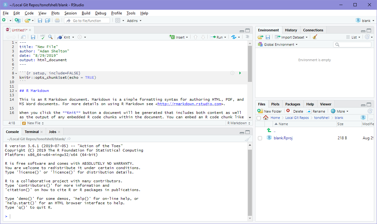
Upper Left Pane - Source

• Shows the source code for your open files
• Each open file gets a tab
• Tabs get different buttons as applicable (like the Run button for R files)

Lower Left Pane - Command Line

• The Console tab shows the R console allowing you to issue and view the output of R commands
• The Terminal tab gives access to the system terminal
• Other tabs appear depending on the context of what you are doing and generally show the statuses of other relevant systems (e.g knitting of an R Markdown document)

Upper Right Pane - Environment et. al.

• The Environment tab shows all the variables in your current environment and allows you to view them
• The History tab shows all the commands you have run this session
• The Connections tab allows you to connect to a database

Lower Right Pane - Everything Else

• The File tab shows files in the current directory and allow for moving, copying, deleting, and renaming files
• The Packages tab allows for the installation, loading, and unloading of packages
• The Help tab provides searchable access to the help files for all installed packages
• The Plots and Viewer tabs display certain objects and files, they are automatically selected when an object to be plotted or viewed is generated

Your First R Script

• Make a new project
  • Go to File > New Project... > New Directory > New Project
  • Give your first project a name, like ‘First Project’
  • Select the folder you want to save this project in
  • Keep all other options unchecked
  • Click Create Project
• Create a new R script
  • Go to File > New File > R Script
  • In the source editor for the script type "Hello world"
  • Save the script under a meaningful name like hello_world
  • In the upper right corner of the source tab, click Run > Run All
  • “Hello world” should print out in the Console tab below
• The Result

## [1] "Hello world"

Variable Assignment

• Assigning a variable allows for that value to be “saved” and referred to later in your code
• It also makes your code more readable, by giving context to what each part is
• Variable names must start with a letter and be followed by an assignment operator (either = or <-)
  • Variable names should be all lower case, with words separated by a period (.) or underscore (_)
  • Both assignment operators work the same, but the equals sign can also refer to other operations in different contexts
  • Which should you use?
    • Using a period in names and <- as an assignment operator is traditional in R, but most other languages do not follow this convention
    • Using underscores in names and equals sign assignment operators is likely more readable to those familiar with other programming languages, but whatever you choose, pick a convention and use it consistently throughout a project
• Just executing the variable name will print out its value(s)

# Create a variable for your favorite number
fav_num = 7
fav.num <- 7

# ...or your favorite color
fav_color = "blue"
fav_color

## [1] "blue"

# Save a vector (a group) of numbers
evens = c(2, 4, 6, 8, 10)

More Things to Try

• Enter each of these into a line in your script and run it or type each into the console and hit enter to run each command individually

# Arithmetic
(2 + 2) * 4^2

## [1] 64

# Use a function
mean(evens)

## [1] 6

# Use variables
fav_num + 3

## [1] 10

fav_num + evens

## [1]  9 11 13 15 17

What did we learn?

• Whether you run a command from a script or the console the result is the same
  • A script is just a way to save a sequence of commands to be reproduced later
• Arithmetic works mostly the way you would expect it to
  • Any expression that returns a result is displayed in the console
• Variables allow you to preserve a value to use later in the session
  • Setting a variable does not return a result, although we can see the value of our variable in the Environment tab or by entering the name of the variable as a command
• Vectors can be created using the c() function and hold any number of the same type of object (e.g all numbers or all text)
• Functions can be applied over vectors
  • However, how they are applied will vary (e.g. mean vs. +)

Data Structures

Vector Basics

• Vectors are a collection of the same type of object, created using the c() function (e.g. c(1, 2, 3) or c("a", "b", "c"))
• Scalars are a single value (e.g. 1 or "a")
  • However in R scalars are just vectors of length one, so 1 is the same as c(1)
• Vectors have two properties
  • A length
  • A type
• While vectors can have any length, there are only six basic types called Atomic Vectors, four of which are commonly used
  • Numeric (e.g. 1 or 5.37)
    • There are two types of numeric vectors
      • Integer (e.g. 1)
      • Double (e.g. 5.37)
  • Character (e.g. "hello" or 'hello')
  • Logical (e.g. TRUE or FALSE)

Working with Vectors

• The c() function can append one vector to another
• Brackets after a reference to a vector will select value(s) at specific indices
  • R is a one-indexed language, meaning the initial value in a vector is stored at index 1

c(c(1,2), c(3,4))

## [1] 1 2 3 4

pets = c("dog", "fish", "cat", "frog", "hamster")
first_pet = pets[1]
first_pet

## [1] "dog"

mammals = pets[c(1,3,5)]
mammals

## [1] "dog"     "cat"     "hamster"

Converting Vectors

• Vectors can be converted to a different compatible type
• Some operations may convert vectors to a compatible type on the fly, called coercion

as.logical(c(1, 0, 0, 1))

## [1]  TRUE FALSE FALSE  TRUE

as.logical(c("TRUE", "FALSE", "F", "T"))

## [1]  TRUE FALSE FALSE  TRUE

as.numeric(c(TRUE, FALSE, F, T))

## [1] 1 0 0 1

as.numeric(c("1", "0", "0", "1"))

## [1] 1 0 0 1

as.character(c(TRUE, FALSE, F, T))

## [1] "TRUE"  "FALSE" "FALSE" "TRUE"

as.character(c(1, 0, 0, 1))

## [1] "1" "0" "0" "1"

sum(c(T, F, T, F))

## [1] 2

Sequences

• A sequence is a special way of generating a numeric vector
• Each item in the vector increases or decreases a constant amount from the previous item
• Sequences can be defined in two ways
  • The seq() function
    • The by argument specifies the amount to increment, by default it is 1
  • The : operator

1:5

## [1] 1 2 3 4 5

seq(1, 5)

## [1] 1 2 3 4 5

seq(1, 10, by = 3)

## [1]  1  4  7 10

Manipulating Character Vectors

• There are some special functions to work with character vectors
• The most notable is paste() which concatenates (combines) multiple character vectors
• There are other built-in functions for working with character vectors, however it is suggested to use their alternatives from the stringr tidyverse package (named after ‘strings’ which is what many other languages call a single-length character vectors)
  • These functions are vectorized and return a list of the results
  • The most used stringr functions are likely str_sub() which returns a portion of a character vector and str_split() which splits a character vector into multiple parts by a sequence of characters

paste("hello", "there", "friends")

## [1] "hello there friends"

paste("hello", "there", "friends", sep = "_")

## [1] "hello_there_friends"

str_sub("grades_2020", start = 8)

## [1] "2020"

str_split("grades_2020", pattern = "_")

## [[1]]
## [1] "grades" "2020"

Making Logical Vectors

• Logical vectors can also be made using different comparison operators including ==, !=, <, >, <=, >=, %in%

1:5 <= 3

## [1]  TRUE  TRUE  TRUE FALSE FALSE

1:5 == 4

## [1] FALSE FALSE FALSE  TRUE FALSE

c("hello", "there", "friend") == "there"

## [1] FALSE  TRUE FALSE

"hello" %in% c("hello", "there", "friend")

## [1] TRUE

Logical Operators

• There are special operators for logical values
  • The ‘and’ operator (&) returns TRUE when two both values evaluate to TRUE
  • The ‘or’ operator (|) returns TRUE when either of two values evaluate to TRUE
  • The ‘not’ operator (!) returns true when a value evaluates to FALSE
• These operations are vectorized

c(TRUE & TRUE, TRUE & FALSE)

## [1]  TRUE FALSE

c(TRUE | TRUE, TRUE | FALSE)

## [1] TRUE TRUE

c(!TRUE, !FALSE)

## [1] FALSE  TRUE

rep(TRUE, 5) & rep(TRUE, 5)

## [1] TRUE TRUE TRUE TRUE TRUE

Finding the Type of a Vector

• Typically R automatically assigns a type to the vector
• You can test the type of a vector using the typeof() function

typeof("hello")

## [1] "character"

typeof(6)

## [1] "double"

typeof(TRUE)

## [1] "logical"

A Vector Inside a Vector

• Other objects are made up vectors
  • Lists
    • A list can contain an unlimited number of vectors or other lists (multi-dimensional)
  • Data-frame / Tibble / Matrix
    • A list of vectors, where each vector is the same length and represents a column of values (two-dimensional)
    • Data-frames or Tibbles can have different types for each column
    • For matrices all columns must be the same type (typically numeric)
• To learn more about vectors and vector-based objects in R for Data Science: Chapter 20

Tibbles

• Data is usually distributed / imported in the form of a data-frame or tibble
  • A tibble is an updated version of the data-frame included in the tidyverse package
    • Tibbles only display the first 10 rows when printed to the console and do not convert column types, unlike data-frames
    • A data-frame can be coerced to a tibble with the as_tibble() function
• Since the tibble is NOT included with the base R packages we must install and load the tidyverse package
  • In the Packages tab there is an Install button, click that and type ‘tidyverse’ and install it
  • Once a package is installed you can load it using the library() function, run library(tidyverse) from a script or the console to load the tidyverse package
  • The tidyverse package is actually several data science packages that follow a common ‘tidy’ analysis philosophy and are all installed and loaded together
    • You can learn more about it on the tidyverse website

Using a Tibble

• Now that the tidyverse package is loaded we can begin to use tibbles for storing data
  • Use the tibble() function to create a new tibble
  • Specify the name and data for each column as a new named argument (e.g. tibble(grades = c("A", "B", "A", "D"), age = age_vector))
    • Notice that you can pass in a variable that refers to a vector that has been previously defined
• Calling the name of a tibble variable prints out the first 10 rows of the tibble
  • View all of the tibble by clicking on its information in the Environment tab
• There are a few ways to select rows and / or columns to view / use
  • Get a column with my_tibble$col_name, select(my_tibble, "col_name"), my_tibble["col_name"], or my_tibble[col_index]
    • Selecting an individual column using the latter two methods will return a tibble NOT a vector
      • For some functions like mean(), you may need to use unlist() to convert a single-columned tibble to a vector
  • Get a row with my_tibble[row_index, ] (notice the comma after row_index)
  • Get a value at a location as a tibble with my_tibble[row_index, col_index]
• Get the dimensions of a tibble with nrow(my_tibble) for the number of rows and ncol(my_tibble) for the number of columns

Trying a Tibble

• The iris data-set gives different measurements for 150 different irises of 3 species
• Create a tibble of the iris data-set using as_tibble(iris) with the variable name iris_data
• Answer the following questions:
  1. What is the mean sepal length?
  2. What is the median petal width?
  3. What is the mean petal area? (Hint: Vectors of same lengths can be multiplied by each other)
  4. Are there an equal number of each species? (Hint: the table() function might be useful)

Trying a Tibble | Answers

iris_data = as_tibble(iris)
mean(iris_data$Sepal.Length)

## [1] 5.843333

median(iris_data$Petal.Width)

## [1] 1.3

mean((iris_data$Petal.Width * iris_data$Petal.Length))

## [1] 5.794067

table(iris_data$Species)

## 
##     setosa versicolor  virginica 
##         50         50         50

Trying a Tibble | Takeaways

• Oftentimes there are many ways to do the same thing
• There are MANY different packages and functions to make your life easier
  • To learn more about a function, package, or included data-set, search for it in the Help tab or, if you know the name, use the ? function (e.g. ?iris)
• The iris data-set contains a special kind of vector for the species variable - called a factor
  • This is essentially a categorical variable
  • Factors have levels (categories) which each have a label assigned to them
  • Can be unordered (as in the case of species) or ordered (as in the case of a Likert scale)

Data Wrangling

What is Data Wrangling?

• The process of taking the data you have and putting it into the form you need for your analysis
• Includes a wide range of processes and tools
  • Importing / converting
  • Variable creation
  • Merging
  • Reshaping
  • Cleaning
• This is usually the most time consuming part of any data project

But First, Some Programming Basics

• Data wrangling can get complex and messy pretty fast
• Functions in R are passed arguments which are the ‘inputs’ of the function
  • Arguments must be passed into the function in the same order they are defined (e.g. for my_function(a, b, c) executing my_function(1, 2, 3) defines a as 1, b as 2, and c as 3)
  • Arguments can be specified in any order if the name of the argument is included with it (e.g. my_function(b = 2, c = 3, a = 1) is the same as before, even though the order does not match the function’s definition)
• In Base R, if you need to use many functions in succession, you have three options
  • Create lots of variables

    a_1 = function_one(x)
    a_2 = function_two(a_2)
    a_3 = function_three(a_3)
    

  • Overwrite existing variables

    a = function_one(x)
    a = function_two(a)
    a = function_three(a)
    

  • Create many nested functions

    a = function_three(function_two(function_one(x)))
    

  • This might be fine for a few operations, but more complex combinations quickly become an unreadable and hard to debug mess
• In research, we want our analyses to be transparent and reproducible, in Base R this is difficult to achieve for complex code
• For these reasons the pipe operator was created and included in the tidyverse

Becoming an R Plumber

• The pipe operator (%>%) directs a variable or the output of a function into the input arguments of another function

So our previous example of

a = function_three(function_two(function_one(x)))

…becomes…

a = x %>% function_one() %>% function_two() %>% function_three()

• Wa-hoo! Much better! But what about functions with multiple arguments, like the round() function (which rounds numbers to a specified amount of decimal places)?

Simple!

round(pi, 3)

## [1] 3.142

…becomes…

pi %>% round(3)

## [1] 3.142

Advanced R Piping

• By default the output is piped into the first argument of the next function
• However, sometimes we might need to pipe data elsewhere
  • The dot (.) tells the pipe where else to pipe the data into, in addition to the first argument

iris_data %>% select(Sepal.Length) %>% as_vector() %>% tibble(Standardized.Length = (. / mean(.)) ) %>% head(1)

## # A tibble: 1 x 2
##       . Standardized.Length
##   <dbl>               <dbl>
## 1   5.1               0.873

• A dot at the beginning of the chain creates a function you can call later

std_var = . %>% as_vector() %>% tibble(Standardized.Var = (. / mean(.)) )
iris_data %>% select(Sepal.Length) %>% std_var() %>% head(1)

## # A tibble: 1 x 2
##       . Standardized.Var
##   <dbl>            <dbl>
## 1   5.1            0.873

• Putting curly brackets ({}) around a function, causes the data to ONLY be piped to the dots

iris_data %>% select(Sepal.Length) %>% as_vector() %>% {tibble(Standardized.Length = (. / mean(.)) )} %>% head(1)

## # A tibble: 1 x 1
##   Standardized.Length
##                 <dbl>
## 1               0.873

• Other pipe operators and functions to pair with pipes exist in the magrittr package

Tidy Data

• Data is easiest to work with when it is tidy, defined by R for Data Science when:
  1. Each variable has its own column.
  2. Each observation has its own row.
  3. Each value has its own cell.
• You will commonly need to convert from long to wide tibbles or vice-versa to tidy data
  • pivot_wider() converts from long data to wide data
  • pivot_longer() converts from wide to long data
  • unite() combines multiple columns into a single new column
  • separate() splits a column into multiple new columns
• Functions from the stringr package can be used to modify character vectors before or after this process

Using pivot_wider()

table2 %>% head(4)

## # A tibble: 4 x 4
##   country      year type          count
##   <chr>       <int> <chr>         <int>
## 1 Afghanistan  1999 cases           745
## 2 Afghanistan  1999 population 19987071
## 3 Afghanistan  2000 cases          2666
## 4 Afghanistan  2000 population 20595360

table2 %>% pivot_wider(names_from = "type", values_from = "count") %>% head(4)

## # A tibble: 4 x 4
##   country      year cases population
##   <chr>       <int> <int>      <int>
## 1 Afghanistan  1999   745   19987071
## 2 Afghanistan  2000  2666   20595360
## 3 Brazil       1999 37737  172006362
## 4 Brazil       2000 80488  174504898

Using pivot_longer()

table1 %>% head(4)

## # A tibble: 4 x 4
##   country      year cases population
##   <chr>       <int> <int>      <int>
## 1 Afghanistan  1999   745   19987071
## 2 Afghanistan  2000  2666   20595360
## 3 Brazil       1999 37737  172006362
## 4 Brazil       2000 80488  174504898

table1 %>% mutate_all(as.character) %>% pivot_longer(cols = everything()) %>% head(4)

## # A tibble: 4 x 2
##   name       value      
##   <chr>      <chr>      
## 1 country    Afghanistan
## 2 year       1999       
## 3 cases      745        
## 4 population 19987071

Using unite()

• Specifying the separator is optional but can be specified with the sep argument (e.g. sep = "_")

table1 %>% head(4)

## # A tibble: 4 x 4
##   country      year cases population
##   <chr>       <int> <int>      <int>
## 1 Afghanistan  1999   745   19987071
## 2 Afghanistan  2000  2666   20595360
## 3 Brazil       1999 37737  172006362
## 4 Brazil       2000 80488  174504898

table1 %>% unite("info", cases, population) %>% head(4)

## # A tibble: 4 x 3
##   country      year info           
##   <chr>       <int> <chr>          
## 1 Afghanistan  1999 745_19987071   
## 2 Afghanistan  2000 2666_20595360  
## 3 Brazil       1999 37737_172006362
## 4 Brazil       2000 80488_174504898

Using separate()

• Specifying the separator is optional but can be specified with the sep argument (e.g. sep = "/")

table3 %>% head(4)

## # A tibble: 4 x 3
##   country      year rate           
##   <chr>       <int> <chr>          
## 1 Afghanistan  1999 745/19987071   
## 2 Afghanistan  2000 2666/20595360  
## 3 Brazil       1999 37737/172006362
## 4 Brazil       2000 80488/174504898

table3 %>% separate(rate, c("cases", "population")) %>% head(4)

## # A tibble: 4 x 4
##   country      year cases population
##   <chr>       <int> <chr> <chr>     
## 1 Afghanistan  1999 745   19987071  
## 2 Afghanistan  2000 2666  20595360  
## 3 Brazil       1999 37737 172006362 
## 4 Brazil       2000 80488 174504898

Excluding Variables

• Commonly in R, the dash (-) is used to specify ‘all but this’, as with
  • Negative indices: my_vector[-5] would return all the items in the vector except the one at index 5
  • Negative variables: my_tibble %>% select(-age) would return a tibble with every variable from my_tibble except age
• Most functions in the tidyverse allow the exclusion of variables from a process by passing their names with a dash in front as the last arguments

table1 %>% head(4)

## # A tibble: 4 x 4
##   country      year cases population
##   <chr>       <int> <int>      <int>
## 1 Afghanistan  1999   745   19987071
## 2 Afghanistan  2000  2666   20595360
## 3 Brazil       1999 37737  172006362
## 4 Brazil       2000 80488  174504898

table1 %>% pivot_longer(cols = -c(country, year), names_to = "type", values_to = "count",) %>% head(4)

## # A tibble: 4 x 4
##   country      year type          count
##   <chr>       <int> <chr>         <int>
## 1 Afghanistan  1999 cases           745
## 2 Afghanistan  1999 population 19987071
## 3 Afghanistan  2000 cases          2666
## 4 Afghanistan  2000 population 20595360

Filtering a Data-set

• Filtering allows to subset data by the specific values of a given variable
• The filter() function takes a comparison of a variable and a value and returns each row where that comparison is TRUE

table1 %>% filter(country == "China")

## # A tibble: 2 x 4
##   country  year  cases population
##   <chr>   <int>  <int>      <int>
## 1 China    1999 212258 1272915272
## 2 China    2000 213766 1280428583

table1 %>% filter(cases > 3000)

## # A tibble: 4 x 4
##   country  year  cases population
##   <chr>   <int>  <int>      <int>
## 1 Brazil   1999  37737  172006362
## 2 Brazil   2000  80488  174504898
## 3 China    1999 212258 1272915272
## 4 China    2000 213766 1280428583

Creating or Modifying Variables

• While there are many ways to create or modify variables, the recommended way is to use the mutate() function
• The mutate() function takes a name for a variable and any code to generate that variable

table1 %>% mutate(rate = cases / population)

## # A tibble: 6 x 5
##   country      year  cases population      rate
##   <chr>       <int>  <int>      <int>     <dbl>
## 1 Afghanistan  1999    745   19987071 0.0000373
## 2 Afghanistan  2000   2666   20595360 0.000129 
## 3 Brazil       1999  37737  172006362 0.000219 
## 4 Brazil       2000  80488  174504898 0.000461 
## 5 China        1999 212258 1272915272 0.000167 
## 6 China        2000 213766 1280428583 0.000167

table1 %>% mutate(year = year %>% as.character() %>% str_sub(3))

## # A tibble: 6 x 4
##   country     year   cases population
##   <chr>       <chr>  <int>      <int>
## 1 Afghanistan 99       745   19987071
## 2 Afghanistan 00      2666   20595360
## 3 Brazil      99     37737  172006362
## 4 Brazil      00     80488  174504898
## 5 China       99    212258 1272915272
## 6 China       00    213766 1280428583

Importing Data

• Most likely the data you need to analyze will not come as a tibble built-in to an R package
• Included in the tidyverse are the readr, haven, and readxl packages for importing different file types directly to tibbles in R
  • readr includes functions to read standard delimited file types such as CSV and TSV files
  • haven includes functions to read files from other stats programs such as Stata, SPSS, and SAS
  • readxl includes functions to read Excel files
• Other packages can add support for reading other types of files
  • sf provides tools for working with GIS data such as shapefiles
  • jsonlite adds functionality for reading and writing to JSONs
  • If it exists, there’s probably an R package to open it
    • However, some packages read data as a data frame and will need to be converted to a tibble before proceeding
• The here() function in the here package makes specifying a file path much easier
  • There is a good example of its benefits and uses on GitHub

Everything Else

• Data-sets are rarely complete, and may be explicitly or implicitly missing values
  • Explicitly missing values are defined in R by NA
  • Oftentimes missing values will need to be omitted, the na.omit() function will remove any rows that have any missing values
  • More about accounting for missing values is covered in this chapter of R for Data Science
• Joining different data-sets is a common problem, but unfortunately it was too time consuming to include here
  • The chapter on relational data, covers this in detail by using data on flights in and out of NYC airports

Analyzing Student Data

1. Download the CSV file student_data.csv and copy it to your project directory
2. Install and import the here package
3. Import the data using the appropriate function from the readr package (learn more about the package on the tidyverse website)
4. Rearrange the data to only have variables for first, middle, and last names, school, year, and math, English, science, and social studies grades
5. Calculate the GPA for each student for each year (Hint: it may be easier to NOT use the mean() function)
6. Find the average GPA for each school in 2018 (This can be done all in one step with the aggregate() function for bonus points)

Analyzing Student Data | Answers

library(here)
student_data = read_csv(here("student_data.csv"))

gathered_student_data = student_data %>% select(-age, -grade_level) %>% 
  pivot_longer(c(-first, -middle, -last, -school), names_to = "key", values_to = "grade") %>%
  separate(key, c("class", "year"), sep = "__") 
gathered_student_data %>% head(4)

## # A tibble: 4 x 7
##   first     middle last   school  class                year  grade
##   <chr>     <chr>  <chr>  <chr>   <chr>                <chr> <dbl>
## 1 Krimhilde Yuri   Hierro Oakwood math_grade           2015     NA
## 2 Krimhilde Yuri   Hierro Oakwood english_grade        2015     NA
## 3 Krimhilde Yuri   Hierro Oakwood science_grade        2015     NA
## 4 Krimhilde Yuri   Hierro Oakwood social_studies_grade 2015     NA

final_student_data = gathered_student_data %>% pivot_wider(names_from = "class", values_from = "grade") %>% 
  mutate(gpa = (math_grade + english_grade + science_grade + social_studies_grade) / 4)
final_student_data %>% head(4)

## # A tibble: 4 x 10
##   first middle last  school year  math_grade english_grade science_grade
##   <chr> <chr>  <chr> <chr>  <chr>      <dbl>         <dbl>         <dbl>
## 1 Krim~ Yuri   Hier~ Oakwo~ 2015          NA            NA            NA
## 2 Krim~ Yuri   Hier~ Oakwo~ 2016          72            64            64
## 3 Krim~ Yuri   Hier~ Oakwo~ 2017          72            58            63
## 4 Krim~ Yuri   Hier~ Oakwo~ 2018          65            57            62
## # ... with 2 more variables: social_studies_grade <dbl>, gpa <dbl>

# the easy way, repeat for each school
final_student_data %>% filter(year == 2018, school == "Oakwood") %>% select(gpa) %>% unlist() %>% mean()

## [1] 60.55165

# the harder way
final_student_data %>% filter(year == 2018) %>% {aggregate(.$gpa, by = list(school = .$school), mean)}

##         school        x
## 1      Oakwood 60.55165
## 2   Pine Field 62.76240
## 3 Shady Willow 66.17926

Communicating Results

Data Visualization

• Aids in the discovery and understanding of relationships in the data
• Data visualization is an essential part of the data science process, and an important method for conveying results, especially to other researchers without data science experience
• In R, there are functions for data visualization in the built-in graphics package, such as the plot() and hist() functions
  • While these can be sufficient for basic visualizations, generating complex visualizations is much more difficult
• In response to this learning curve Hadley Wickham, author of most of the tidyverse packages, created ggplot2 a data visualization package which follows a ‘grammar of graphics’
  • ggplot2 is one of the world’s most popular data visualization tools, used by world renowned organisations such as the New York Times and FiveThirtyEight, and has been downloaded millions of times
  • Its simplicity in building and customizing visualizations is desirable to amateurs and professionals alike, and numerous packages have expanded its philosophy to other aspects of data visualization

ggplot2 Basics

• ggplot2 layers components on top of each other to build a visualization
• The process is started with the ggplot() function which specifies a data source and any default aesthetic mappings or settings to use
  • ggplot() accepts data in data frame or tibble form
  • Aesthetic mappings, generated with the aes() function, connect a dimension of data to a dimension of the visualization
• Next comes one or more geometry layers, each corresponding to a type of visualization to include
  • Each additional geometry layer can inherit the default aesthetic mappings and settings, if possible, or specify different ones
• Other layers can be added to adjust other parameters, such as facets, labels, scales, and themes
• All of these layers are linked together to form one visualization using the addition operator(+)

Making a Simple Visualization

1. Select a data source - this can be piped in, which is useful if the data needs to be wrangled into the correct form for the visualization
2. Specify default aesthetic mappings - x, y, color, and fill are the most common, but some geometries will use more or only a portion of these
3. Select a geometry function (or several) - each of these are prefaced by geom_ (e.g. geom_point())
4. Save to a variable to add more layers or view later

displ_year_plot = ggplot(mpg, aes(x = displ, y = hwy)) + geom_point()
displ_year_plot

Making a Slightly Less Simple Visualization

• Specifying color in an aesthetic maps changes in color based to a variable, creating a legend
• Specifying color in a geometry simply sets the same color for all elements in that geometry

displ_year_plot = ggplot(mpg, aes(x = displ, y = hwy)) + geom_point(aes(color = class))
displ_year_plot

displ_year_plot + geom_smooth(color = "grey60")

Making a Complicated Visualization

• Functions prefixed in scale_ can alter the scale used for a specific dimension
  • Here scale_radius() adjusts the size aesthetic by the radius, the default scale_size() adjusts the area
• The labs() function allows for the definition of labels
• A facet arranges multiple visualizations which each use a different subset based on a variable
• Themes alter the position, size, and other attributes of objects
• This is probably a bad visualization because too much has been stuffed into it

mpg %>% arrange(-cyl) %>% ggplot(aes(x = displ, y = hwy)) + 
  geom_point(aes(color = class, size = cyl)) + 
  geom_smooth(color = "grey60") + 
  scale_radius(range = c(2, 7)) + 
  facet_wrap(~ year) + theme(legend.position = "bottom") + 
  labs(title = "Cars with Larger Engines get Worse Fuel Efficiency", subtitle = "At highway speeds in both 1999 and 2008", 
       x = "Engine Displacement  (L)", y = "Highway Fuel Efficiency (mpg)", color = "Vehicle \nClass", size = "Number of \nCylinders")

Introduction to R Markdown

• R scripts are great for saving code, but if you want to make a document or report, it involves a tedious process of exporting results to be inserted into a Word or Latex document
• R Markdown attempts to solve this problem by combining R code with a formatted document
• R Markdown code can still be easily read while also allowing for detailed formatting options
• R Markdown files are ‘knitted’ into a common document type such as HTML (webpage), PDF, Word document, and others (this presentation was completely made with R Markdown!)
• It allows for a completely reproducible document of which any changes can easily be tracked by version control software - ideal for research purposes
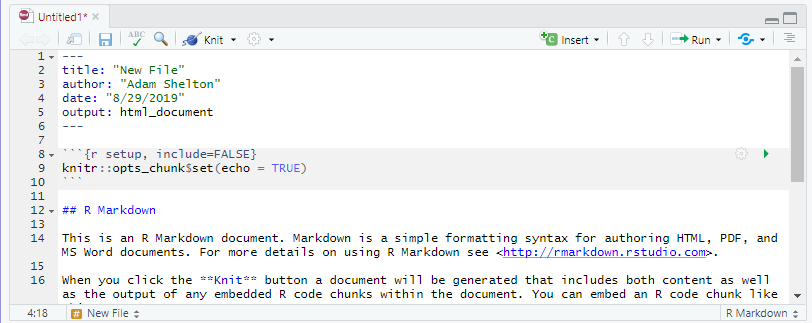
• A R Markdown file is broken into three basic parts
  • The header defines a title, author, and date, as well as the options for knitting into a final document
  • Markdown sections allow for rich formatted text
  • Code blocks allow for sections of code, where the code and output can be made viewable in the final knitted document

Making an R Markdown document

• R Studio will generate a blank R Markdown file with some basic parts by selecting R Markdown from the File > New File... menu
  • A dialog box will give you some basic options for your R Markdown file
• Create a new code block by pressing Ctrl + Alt + i or on macOS Cmd + Opt + i
• Name a code block by adding a space and a name after the r in the code block header (e.g. {r code-block-name})
• The gear to the right of the code block gives options for displaying code and/or the output of code
• The play button allows for an individual code block to be run, or all code blocks can be run from the Run menu
  • When the R Markdown file is knitted all the code blocks are run except for any that are cached (learn about caching and other code block options here)

Basic Markdown

• R Markdown is based off of Markdown which is a basic syntax markup language for formatting text
• A line of header text is started with an octothorp (#) followed by a space (e.g. # My Big Fancy Header)
  • Subheadings can be created by adding more octothorps

    # Main Heading 1
    ## Sub-heading 1.1
    ### Sub-heading 1.1.1
    

• Unordered lists can be made by starting each line with a dash (-), asterisk, (*), or addition signs (+) followed by a space
• Ordered lists can be made by starting each line with a number and a period (e.g 1.) followed by a space
  • The number you use does not matter, R changes it to the correct number if it is wrong
• Text can be italicized by surrounding it in single asterisks or underscores (e.g. *italics* or _also italics_)
• Text is bolded by surrounding it in double asterisks or underscores (e.g. **bold** or __also bold__)
  • Combine them to do both (e.g. __*bold and italics*__)
• Strikethrough text can be displayed by using double tildes (e.g. ~~strikethrough~~)
• Make a horizontal rule by placing three or more hyphens, asterisks, or underscores on a line

Links and Things

• Links can be made with a display text surrounded by square brackets followed by the URL surrounded by a set of parentheses (e.g. [A Link to Google](http://google.com)) A Link to Google
• Pictures can be added in a similar manner but an exclamation mark is added first (e.g ![A Cat Picture](/r-crash-course/cat_picture.jpg))
• Links and pictures can be linked to a file on your computer, the web, or even to another section of the document.
• R Markdown can do a lot more! The free eBook R Markdown: The Definitive Guide, spills all of its secrets

Visualizing Student Data

Create an R Markdown document knitted into HTML with visualizations to answer the following questions:

1. Is one school overrepesented in the data-set?
2. Is there a relationship between math and English grades?
3. Which school has the highest GPAs?
4. Do grades by subject vary by school?

Visualizing Student Data | Answers

final_student_data %>% ggplot(aes(x = school)) + geom_bar()

final_student_data %>% ggplot(aes(x = math_grade, y = english_grade, color = school)) + geom_point() + geom_smooth(color = "grey60")

final_student_data %>% ggplot(aes(x = school, y = gpa, fill = school)) + geom_violin()

gathered_student_data %>% ggplot(aes(x = school, y = grade, fill = school)) + geom_violin() + facet_wrap(~class)

Programming

Programming in R

• R is not only a statistical environment but a programming language
  • While R is not a general purpose programming language like Python or Java, it has many of the same components
• In certain circumstances the print() function may be necessary to print to the console
  • In most loops or functions only the print() function outputs to the console, in contrast to the rest of
• R is an interpreted language which means the R console must convert R code into a language that the operating system can understand
• R code can include comments, lines are not executed that explain what code does, by starting a line with an octothorp (#)

if Statement

• An if statement executes code if a logical condition evaluates to true

grade_level = 12

if (grade_level > 8) {
  print("high school")
}

## [1] "high school"

if else Statement

• An if else statement executes a section of code if a logical condition evaluates to true, or a different section of code if it does not
  • ``if else` statements can be strung together to test for multiple conditions

grade_level = 7

if (grade_level > 8) {
  print("high school")
} else if(grade_level > 5) {
  print("middle school")
} else {
  print("elementary school")
}

## [1] "middle school"

while Loops

• while loops continue to run a section of code as long as a logical condition continues to evaluate to true
  • If the condition will always evaluate to be true, then the code will run forever without manual intervention
• Conducting data analysis tasks in R do not usually use while loops

grade_level = 6
while (grade_level < 12) {
  print(grade_level)
  grade_level = grade_level + 1
}

## [1] 6
## [1] 7
## [1] 8
## [1] 9
## [1] 10
## [1] 11

for Loops

• for loops in R are technically for each loops which loop a section of code for every element in a vector
  • A local variable is defined which contains the value of the current object for each iteration
• This process of looping through data is commonly used in data analysis

for (cur_grade_level in 6:12) {
  print(cur_grade_level)
}

## [1] 6
## [1] 7
## [1] 8
## [1] 9
## [1] 10
## [1] 11
## [1] 12

The apply Family

• The apply family corresponds to the apply(), lapply(), and sapply() functions which execute a function for each element in a vector or list
• This is the preferred alternative to using for loops in R

Performance Comparisons

• for loops in R, while intuitive due to their similarity to other languages, are not the best for performance
• Wherever possible, loops should be avoided for vectorized operations
• If vectorized functions do not exist to complete the intended task, an apply function should be used

library(tictoc)
rand_numbers = runif(10^6, 0, 10) %>% matrix(ncol = 1000) %>% as_tibble()

## Warning: `as_tibble.matrix()` requires a matrix with column names or a `.name_repair` argument. Using compatibility `.name_repair`.
## This warning is displayed once per session.

tic()
output = double(nrow(rand_numbers))
for (i in 1:nrow(rand_numbers)) {
  output[i] = rand_numbers[i, ] %>% unlist() %>% mean()
}
toc()

## 1.53 sec elapsed

tic()
output = apply(rand_numbers, 1, mean)
toc()

## 0.06 sec elapsed

tic()
output = rowMeans(rand_numbers)
toc()

## 0.02 sec elapsed

Functions

• Functions allow the repetition of code efficiently
  • Generally if a section of code is copied and pasted more than twice, it should be turned into a function
• Functions not only save time, they make code easier to read and understand
• Debugging also becomes easier, and if there is a bug in the function, fixing it once fixes it in every place the function is called
• Functions have 4 parts
  • Function (variable) name
  • Argument(s)
  • Function body
  • Return statement (optional)

Starting a Function

• A function is defined like any other variable with a variable name which is set to a value, in this case a function() (e.g. function_name = function())
• Just like already-made functions, arguments are passed to the function by variable names inside the parentheses
  • Unlike using a function, these arguments create variables to be referenced inside the function
• Curly brackets define the body of the function, where the lines of code that make the function go

my_function = function(argument1, argument2) {
  # adds argument1 and argument2
  result = argument1 + argument2
}

More About Arguments

• The values stored in arguments are only available inside the function
• Any argument with the same name of an existing variable overrides the value of the variable that already exists
• An argument can be made optional by setting a ‘default’ value with the = operator
• The ellipses (...) operator allows unlimited additional arguments to be passed into the function

a = 3
# ... passes additional arguments to the print function
do_something_weird = function(a, ..., b = 5) {
  print(rep(a, times = b), ...)
}

do_something_weird(1)

## [1] 1 1 1 1 1

do_something_weird(9, 7)

## [1] 9 9 9 9 9

do_something_weird(5.63, digits = 1)

## [1] 6 6 6 6 6

Ending a Function

• Since any variables or data created within a function are not available from the rest of the R script, data must be passed back to the script or the user
  • Data can be printed to the console using the print() function
  • Data can be returned to the r script using the return() function, which also exits the function when it is called
• Returned data can be saved to a variable or passed along a pipe to another function

# now returns the value instead of printing it to the console
do_something_weird = function(a, ..., b = 5) {
  return(rep(a, times = b, ...))
}

ones = do_something_weird(1)
ones

## [1] 1 1 1 1 1

do_something_weird(9, 7) %>% sum()

## [1] 63

Converting Grades

• Create a function that can convert 100 point numeric grades and 4 point numeric grades to letter grades (no pluses or minuses)
• The first argument should take a vector of grade(s), with additional arguments as you see fit
• Easily vectorize a function using the Vectorize() function
• Functions can be nested in another function if necessary
• Bonus points if you check for errors and use the warning() or stop() functions to convey that something has gone wrong, or the message() when something else has happened

Converting Grades | Answer

convert_grade = function(grade, input_type = "default") {
  grade = as.vector(unlist(grade))
  if (min(grade) < 0 | !is.numeric(grade)) stop("Invalid grade")
  
  if (input_type == "default") {
    if (max(grade) < 4) {
      input_type = "four"
      message("Converting to 4 point scale")
    } else {
      input_type = "hundred"
      message("Converting to 100 point scale")
    }
  }
  
  conv_gr = Vectorize(function(grade, input_type) {
    if (input_type == "hundred") {
      if (grade > 100) stop("Invalid grade")
      if (grade > 89) return("A")
      if (grade > 79) return("B")
      if (grade > 69) return("C")
      if (grade > 59) return("D")
      return("F")
    }
    if (input_type == "hundred") {
      if (grade > 4) stop("Invalid grade")
      if (grade > 3.7) return("A")
      if (grade > 2.7) return("B")
      if (grade > 1.7) return("C")
      if (grade > 1.0) return("D")
      return("F")
    }
  })
  
  return(conv_gr(grade, input_type))
}

student_data %>% select(math_grade__2018) %>% convert_grade()

## Converting to 100 point scale

##   [1] "D" "C" "D" "B" "D" "F" "B" "C" "D" "D" "D" "C" "D" "F" "C" "D" "C" "C"
##  [19] "C" "D" "D" "B" "C" "D" "D" "C" "C" "F" "D" "D" "D" "C" "C" "D" "B" "C"
##  [37] "D" "C" "C" "B" "D" "D" "C" "D" "C" "C" "F" "C" "B" "D" "A" "C" "F" "F"
##  [55] "F" "D" "C" "F" "F" "B" "D" "C" "C" "C" "F" "D" "D" "D" "C" "D" "C" "C"
##  [73] "B" "B" "D" "C" "C" "C" "F" "D" "C" "C" "D" "F" "D" "C" "C" "D" "B" "B"
##  [91] "B" "C" "D" "C" "F" "D" "B" "C" "C" "D" "C" "D" "D" "C" "A" "B" "D" "C"
## [109] "D" "D" "B" "C" "B" "F" "D" "C" "B" "B" "D" "C" "B" "D" "C" "D" "C" "C"
## [127] "C" "F" "F" "D" "C" "C" "D" "C" "C" "B" "C" "F" "C" "C" "C" "B" "C" "D"
## [145] "D" "F" "B" "B" "B" "C" "D" "D" "D" "C" "C" "B" "C" "D" "C" "B" "B" "A"
## [163] "C" "D" "D" "C" "D" "D" "C" "B" "C" "A" "D" "D" "C" "D" "F" "C" "D" "F"
## [181] "C" "C" "D" "D" "D" "D" "C" "F" "C" "D" "C" "C" "C" "B" "B" "C" "D" "D"
## [199] "D" "F" "C" "C" "D" "C" "C" "C" "C" "D" "B" "C" "B" "C" "D" "C" "F" "C"
## [217] "D" "F" "A" "B" "D" "D" "C" "C" "F" "D" "D" "C" "C" "D" "F" "C" "C" "D"
## [235] "C" "D" "D" "B" "F" "B" "F" "D" "D" "C" "C" "C" "D" "C" "B" "C" "D" "F"
## [253] "C" "F" "C" "D" "D" "D" "C" "D" "D" "C" "D" "D" "C" "D" "C" "C" "C" "C"
## [271] "D" "D" "C" "D" "C" "A" "D" "D" "F" "D" "C" "D" "C" "F" "D" "C" "D" "C"
## [289] "B" "C" "A" "C" "D" "C" "F" "F" "D" "C" "A" "C" "B" "B" "C" "D" "F" "B"
## [307] "C" "C" "D" "D" "C" "D" "B" "B" "C" "C" "C" "D" "D" "B" "D" "C" "C" "C"
## [325] "C" "B" "B" "C" "B" "D" "B" "D" "D" "B" "F" "C" "F" "B" "F" "B" "D" "D"
## [343] "C" "D" "C" "D" "D" "A" "D" "F" "C" "A" "C" "C" "C" "D" "D" "A" "C" "D"
## [361] "C" "C" "F" "C" "F" "A" "D" "C" "C" "D" "F" "F" "C" "C" "B" "D" "C" "B"
## [379] "B" "B" "F" "B" "C" "D" "C" "C" "B" "B" "A" "B" "C" "C" "C" "D" "F" "B"
## [397] "B" "C" "C" "C" "C" "D" "D" "D" "D" "B" "B" "C" "D" "D" "C" "B" "D" "C"
## [415] "D" "C" "B" "C" "F" "D" "D" "D" "D" "D" "F" "C" "D" "C" "F" "D" "C" "B"
## [433] "C" "D" "F" "B" "D" "D" "C" "D" "D" "C" "C" "D" "B" "C" "C" "D" "C" "C"
## [451] "C" "D" "D" "D" "D" "C" "D" "C" "F" "F" "D" "F" "C" "B" "D" "D" "B" "D"
## [469] "B" "C" "C" "C" "B" "F" "A" "C" "D" "C" "F" "F" "D" "F" "D" "C" "C" "D"
## [487] "B" "C" "C" "C" "D" "B" "C" "C" "D" "C" "F" "C" "C" "C"

convert_grade(103)

## Converting to 100 point scale

## Error in (function (grade, input_type) : Invalid grade

Wrapping Up

• R provides a wide range of tools for every part of the data analysis process
• While hopefully this presentation has been a useful resource for learning about R, a myriad of free and fantastic resources exist online
• R has its own unique quirks and features, but many of the underlying skills translate to other programming languages, especially Python
  • Python code can even be run from within R, for those times when Python is the better suited tool for the job